
Pop Music Random Forest Classifier with Spotify
Supervised Learning Techniques: Background
Supervised learning is a machine learning technique where a model learns from labeled data. Since every data input is paired with a corresponding output label, the model can iteratively test various weights and optimize those weights using the known ‘correct’ prediction. This allows the model to pull out complicated patterns from historical data with the goal of predicting the output for new, unseen data.
Contrast this with unsupervised learning where the model uses unlabeled data to find patterns without explicit guidance. Unsupervised learning techniques such as clustering are commonly employed to uncover hidden relationships or groupings of data that can then be used to reduce the number of features in a dataframe while preserving important information.
- Supervised Learning Techniques: Background
- Supervised Learning Models
- Tree-Based Models
- Predicting Popularity with a Random Forest: An Example
- Conclusion
Supervised Learning Models
Common types of supervised learning models include:
- Linear Regression:
- Used for predicting a continuous outcome variable based on one or more input features. Applications include sales forecasting, stock price prediction, and house price estimation.
- Logistic Regression:
- Primarily used for binary classification tasks, where the output variable has two possible outcomes. Applications include spam detection, disease diagnosis, and credit risk assessment.
- Decision Trees:
- These models partition the feature space into regions and make predictions based on the majority class or average value within each region. They’re used in various applications, including customer segmentation, fraud detection, and medical diagnosis.
- Random Forests:
- An ensemble learning method that combines multiple decision trees to improve predictive performance and reduce overfitting. Common applications include recommendation systems, financial forecasting, and image classification.
- Support Vector Machines (SVM):
- Used for both classification and regression tasks by finding the hyperplane that best separates the classes or fits the regression line. Applications include text classification, image recognition, and medical diagnosis.
- Naive Bayes:
- A probabilistic classifier based on Bayes’ theorem with strong independence assumptions between features. It’s commonly used in spam filtering, sentiment analysis, and document categorization.
- Neural Networks:
- Deep learning models composed of interconnected layers of nodes that mimic the structure and function of the human brain. They’re used in a wide range of applications, including image recognition, natural language processing, and autonomous driving.
Supervised learning techniques have wide ranging applications including healthcare, finance, marketing and e-commerce, and can be used wherever there is a need to make predictions or classify data based on historical examples.
Tree-Based Models
A decision tree is a supervised machine learning model with a hierarchical structure composed of nodes and branches; each internal node represents a decision based on a feature, and each branch represents the outcome of that decision. The leaf nodes represent the final predictions or classifications.
To generate predictions, the algorithm applies optimal, recursive binary splits (called decision rules) to the features in a dataframe to either maximize information gain or minimize impurity (i.e heterogeneity) at each node.
For classification tasks (categorical outcomes), the leaf nodes represent class labels and the prediction is the majority class in that node. In regression (numerical outcomes), the leaf nodes represent average values of the target variable and the prediction is the average value for the subset of data based on the node’s decision rule.
Random Forests
A Random Forest is an ensemble model (a model that combines several models) made up of multiple decision trees created from various subsets of the training data; the resulting model predictions are aggregated across all trees. Results from a random forest algorithm are more accurate, stable and generalizable compared to results from a single decision tree. Additionally, random forests provide measures of feature importance (the strength of the effect of each feature in the algorithm) which improves model interpretability.
Boosting
Boosting is another ensemble learning technique that uses multiple decision tree models. Unlike random forests that build multiple independent trees in parallel, boosting builds trees sequentially, with each tree learning from the mistakes of its predecessors.
Boosting is known for its ability to achieve high predictive accuracy, especially in scenarios where there are complex relationships between features and the target variable. However, boosting algorithms are more prone to overfitting compared to random forests and can be computationally expensive due to their sequential nature.
Steps to Create a Model
The following is a brief overview of the steps for creating and evaluating a random forest model:
- Visualize features and calculate descriptive statistics:
- Plot data to examine distributions and relationships between features.
- Split your dataframe into a training dataset and a test dataset (and optionally, a validation dataset):
- Set aside a subsample of your data to evaluate the accuracy of the trained model
- Instantiate model, select features and tune hyperparameters:
- Most models allow users to specify some details (called hyperparameters) of the learning process. The model accuracy can be improved by making and testing small changes to these hyperparameters. Additionally the model can be improved by removing non-relevant features. Feature relevancy can be determined by calculating loss metric increase or decrease with the removal/addition of each individual feature to the model.
- Model evaluation:
- Common metrics used for evaluating classification models include accuracy, precision, recall, F1-score, and area under the ROC curve (AUC-ROC). Additionally, a confusion matrix can provde a detailed breakdown of the model’s predictions by showing the number of true positives, true negatives, false positives, and false negatives. For regression models, metrics such as mean squared error (MSE), mean absolute error (MAE), and R-squared are commonly used.
- Perform cross validation:
- Cross validation compares training versus testing accuracy to determine if the model is overfit (i.e will the model be accurately generalizable to new data). In k-fold cross-validation, the dataset is divided into k subsets (folds) and trained k times, each time using k-1 folds for training and the remaining fold for validation. This allows for more robust estimation of model performance.
- Save the model:
- Model can be exported and saved to generate predictions on new data.
Summary
Tree-based models are broadly applicable, intuitive and interpretable models that are widely used for their simplicity and effectiveness in handling both categorical and numerical data. They are an ideal choice for tasks where large, tabular data frames with historical data are available because the algorithm can capture complicated interactions within data and, unlike other broadly applicable techniques like linear or logistic regression, they don’t require normally distributed error or monotonic relationships between variables to be effective.
Predicting Popularity with a Random Forest: An Example
The following example uses the scikit-learn python package and Spotify data available for download here: https://www.kaggle.com/datasets/thedevastator/spotify-tracks-genre-dataset/data to create a random forest model for predicting song popularity.
Import packages and load data.
import pandas as pd
import matplotlib.pyplot as plt
import plotly.express as px
import plotly.graph_objects as go
from plotly.subplots import make_subplots
import numpy as np

from catboost import Pool, cv

from sklearn.model_selection import KFold
from sklearn.model_selection import cross_val_score
from sklearn.model_selection import train_test_split
from sklearn.ensemble import RandomForestClassifier
from sklearn.ensemble import GradientBoostingRegresso
from sklearn.preprocessing import OneHotEncoder
from sklearn.preprocessing import MinMaxScaler
from sklearn.metrics import ConfusionMatrixDisplay
from sklearn.metrics import mean_absolute_percentage_error
from sklearn.metrics import mean_squared_error
from sklearn.metrics import r2_score
from sklearn.metrics import classification_report
from sklearn.metrics import confusion_matrix

music_data = pd.read_csv('/content/drive/MyDrive/online learning/projects/spotify_random_forest/train.csv')
Data Preparation
Examine descriptive statistics and check for missing values.
na_cols=music_data.columns[music_data.isna().any()].tolist()

# Missing values summary
mv=pd.DataFrame(music_data[na_cols].isna().sum(), columns=['Number_missing'])

desc = pd.DataFrame(index = list(music_data))
desc['count'] = music_data.count()
desc['nunique'] = music_data.nunique()
desc['%unique'] = desc['nunique'] / len(music_data) * 100
desc['null'] = music_data.isnull().sum()
desc['Percentage_missing']=np.round(100*mv['Number_missing']/len(music_data),2)
desc['type'] = music_data.dtypes
desc = pd.concat([desc, music_data.describe().T.drop('count', axis = 1)], axis = 1)
desc
| count | nunique | %unique | null | Percentage_missing | type | mean | std | |
|---|---|---|---|---|---|---|---|---|
| Unnamed: 0 | 114000 | 114000 | 100.000000 | 0 | NaN | int64 | 56999.500000 | 32909.109681 |
| track_id | 114000 | 89741 | 78.720175 | 0 | NaN | object | NaN | NaN |
| artists | 113999 | 31437 | 27.576316 | 1 | 0.0 | object | NaN | NaN |
| album_name | 113999 | 46589 | 40.867544 | 1 | 0.0 | object | NaN | NaN |
| track_name | 113999 | 73608 | 64.568421 | 1 | 0.0 | object | NaN | NaN |
| popularity | 114000 | 101 | 0.088596 | 0 | NaN | int64 | 33.238535 | 22.305078 |
| duration_ms | 114000 | 50697 | 44.471053 | 0 | NaN | int64 | 228029.153114 | 107297.712645 |
| explicit | 114000 | 2 | 0.001754 | 0 | NaN | bool | NaN | NaN |
| danceability | 114000 | 1174 | 1.029825 | 0 | NaN | float64 | 0.566800 | 0.173542 |
| energy | 114000 | 2083 | 1.827193 | 0 | NaN | float64 | 0.641383 | 0.251529 |
| key | 114000 | 12 | 0.010526 | 0 | NaN | int64 | 5.309140 | 3.559987 |
| loudness | 114000 | 19480 | 17.087719 | 0 | NaN | float64 | -8.258960 | 5.029337 |
| mode | 114000 | 2 | 0.001754 | 0 | NaN | int64 | 0.637553 | 0.480709 |
| speechiness | 114000 | 1489 | 1.306140 | 0 | NaN | float64 | 0.084652 | 0.105732 |
| acousticness | 114000 | 5061 | 4.439474 | 0 | NaN | float64 | 0.314910 | 0.332523 |
| instrumentalness | 114000 | 5346 | 4.689474 | 0 | NaN | float64 | 0.156050 | 0.309555 |
| liveness | 114000 | 1722 | 1.510526 | 0 | NaN | float64 | 0.213553 | 0.190378 |
| valence | 114000 | 1790 | 1.570175 | 0 | NaN | float64 | 0.474068 | 0.259261 |
| tempo | 114000 | 45653 | 40.046491 | 0 | NaN | float64 | 122.147837 | 29.978197 |
| time_signature | 114000 | 5 | 0.004386 | 0 | NaN | int64 | 3.904035 | 0.432621 |
| track_genre | 114000 | 114 | 0.100000 | 0 | NaN | object | NaN | NaN |
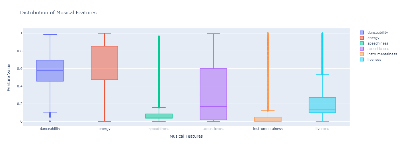
Plot distributions for variables with the same scale.
features = ['danceability', 'energy', 'speechiness', 'acousticness', 'instrumentalness', 'liveness']

# Plotting the distributions of these features
fig = go.Figure()
for feature in features:
    fig.add_trace(go.Box(y=music_data[feature], name=feature))

fig.update_layout(
    title="Distribution of Musical Features",
    yaxis_title="Feature Value",
    xaxis_title="Musical Features"
)

fig.show()
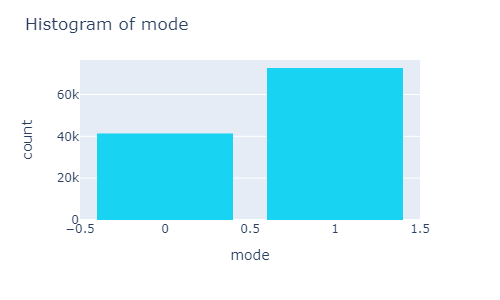
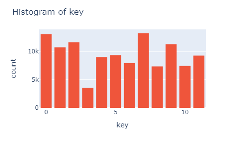
Create histogram function to plot additional variables.
def plot_histogram(data, x, y=None):
    """
    Plot a histogram with random colors using Plotly.

    Parameters:
    - data: DataFrame
    - x: str, column name for the x-axis
    - y: str, optional, column name for the y-axis (default is None)
    """
    # Check if y is provided for a 2D histogram
    if y:
        color_sequence = np.random.choice(px.colors.qualitative.Plotly, size=1)[0]
        fig = px.histogram(data, x=x, y=y, color_discrete_sequence=[color_sequence])
        fig.update_layout(title=f'2D Histogram of {x} and {y}', xaxis_title=x, yaxis_title=y, bargap=0.2, autosize=False, width=500, height=300)
    else:
        # Plot a 1D histogram with random colors
        color_sequence = np.random.choice(px.colors.qualitative.Plotly, size=1)[0]
        fig = px.histogram(data, x=x, color_discrete_sequence=[color_sequence])
        fig.update_layout(title=f'Histogram of {x}', xaxis_title=x, bargap=0.2, autosize=False, width=500, height=300)

    fig.show()
plot_histogram(music_data, x='explicit')
plot_histogram(music_data, x='mode')
plot_histogram(music_data, x='track_genre')
plot_histogram(music_data, x='time_signature')
plot_histogram(music_data, x='key')
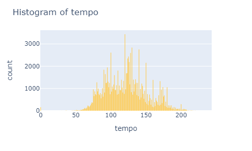
plot_histogram(music_data, x='tempo')
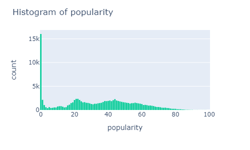
plot_histogram(music_data, x='popularity')

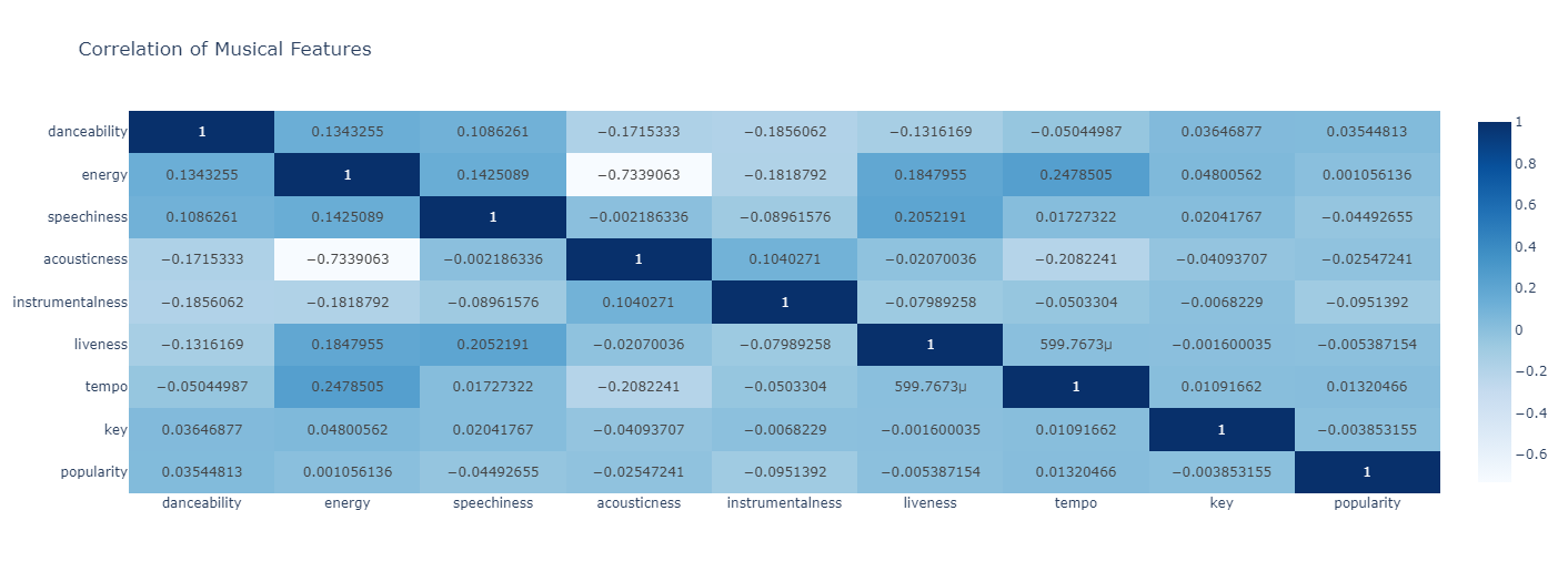
Plot correlations.
attributes = [
'danceability', 'energy', 'speechiness', 'acousticness', 'instrumentalness', 'liveness', 'tempo', 'key', 'popularity'
]

# correlation matrix for the selected attributes
correlation_matrix = music_data[attributes].corr()

# heatmap to visualize the correlation matrix
fig = px.imshow(correlation_matrix,
                x=attributes,
                y=attributes,
                text_auto=True,
                aspect="auto",
                color_continuous_scale='Blues',
                title='Correlation of Musical Features')

# layout to put the x-axis labels at the bottom
fig.update_xaxes(side="bottom")

# Show the figure
fig.show()
Model Selection Process: CatBoost
I tested both the GradientBoostingRegressor and the GradientBoostingClassifier model from sklearn which resulted in and R-squared of .27 and an accuracy of about 75%, respectively. Examining feature importances indicated that track_genre was a strong predictor so I decided to test performance of the CatBoostRegressor and CatBoostClassifier. CatBoost is an open source library for a gradient boosting algorithm developed by Yandex et al in 2017 specifically for native processing categorical features. Using CatBoost, the regression R-squared increased to .35 and the classification accuracy was bumped up to 82%. The following code is for the generation of the CatBoostClassifier model.
Model Creation
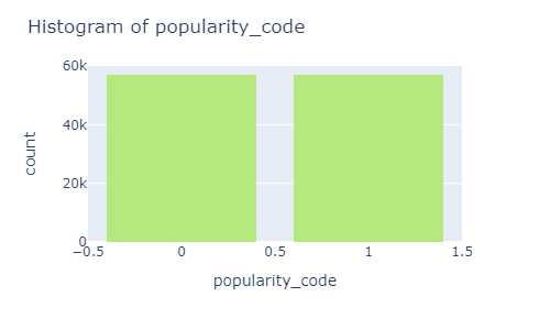
Created binary popularity variable.
music_data['popularity_code'] = np.where(music_data['popularity'] < 35, 0, 1)
plot_histogram(music_data, x='popularity_code')
 >
>
Create training dataframe, testing dataframe and instantiate model.
dataframe = music_data[['popularity_code', 'duration_ms', 'explicit', 'danceability', 'energy', 'key', 'loudness', 'mode', 'speechiness', 'acousticness', 'instrumentalness',
 'liveness', 'valence', 'tempo', 'time_signature', 'track_genre']]

X = dataframe.loc[:, dataframe.columns != 'popularity_code']
y = dataframe.loc[:, dataframe.columns == 'popularity_code']

#create traing and testing set
X_train, X_test, y_train, y_test = train_test_split(X, y, test_size=0.3, random_state=13)

categorical_features = ['explicit', 'track_genre']

train_dataset = Pool(X_train, y_train, categorical_features)
test_dataset = Pool(X_test, y_test, categorical_features)

model = cb.CatBoostClassifier()
Hyperparameter tuning using GridSearch.
grid = {'iterations': [500, 800],
        'learning_rate': [0.03, 0.1],
        'depth': [6, 8],
        'l2_leaf_reg': [4, 5]}

model.grid_search(grid, train_dataset)
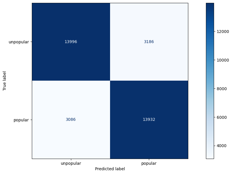
Model Evaluation
Generate classification report and confusion matrix for model.
y_pred = model.predict(X_test)

print(classification_report(y_test, y_pred))

disp = ConfusionMatrixDisplay(confusion_matrix=confusion_matrix(y_test, y_pred), display_labels=["unpopular", "popular"])
disp.plot(cmap="Blues", values_format="d")
plt.show()

| precision | recall | f1-score | support | |
|---|---|---|---|---|
| unpopular | 0.82 | 0.82 | 0.82 | 17182 |
| popular | 0.82 | 0.82 | 0.82 | 17018 |
| accuracy | 0.82 | 34200 | ||
| macro avg | 0.82 | 0.82 | 0.82 | 34200 |
| weighted avg | 0.82 | 0.82 | 0.82 | 34200 |
The following metrics are defined as:
- Precision:
- Ratio of true positive predictions to the total number of positive predictions made by the model.
- TP / (TP + FP), where TP is the number of true positives and FP is the number of false positives.
- Recall (sensitivity or true positive rate):
- Ratio of true positive predictions to the total number of actual positive instances in the dataset.
- TP / (TP + FN), where TP is the number of true positives and FN is the number of false negatives.
- F1-Score:
- Harmonic mean of precision and recall, providing a single metric that balances both precision and recall. It is calculated as 2 * (precision * recall) / (precision + recall). The F1-score ranges from 0 to 1, where a higher value indicates better overall performance.
- Support:
- The number of occurrences of each class in the true labels. It provides context for the precision, recall, and F1-score metrics by showing the distribution of true instances across different classes.
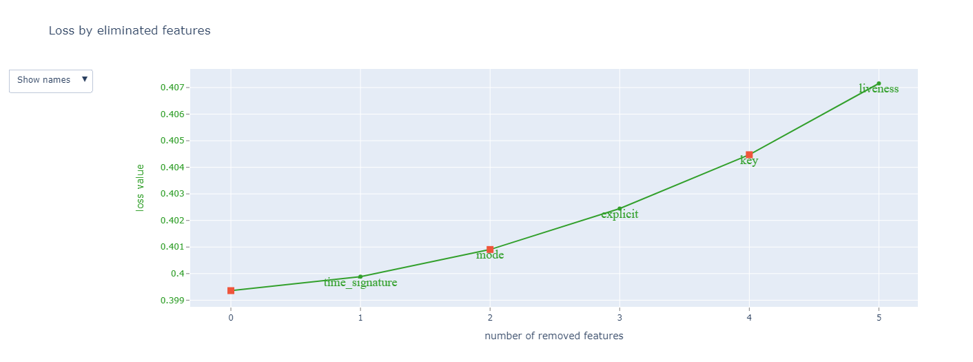
Feature Selection
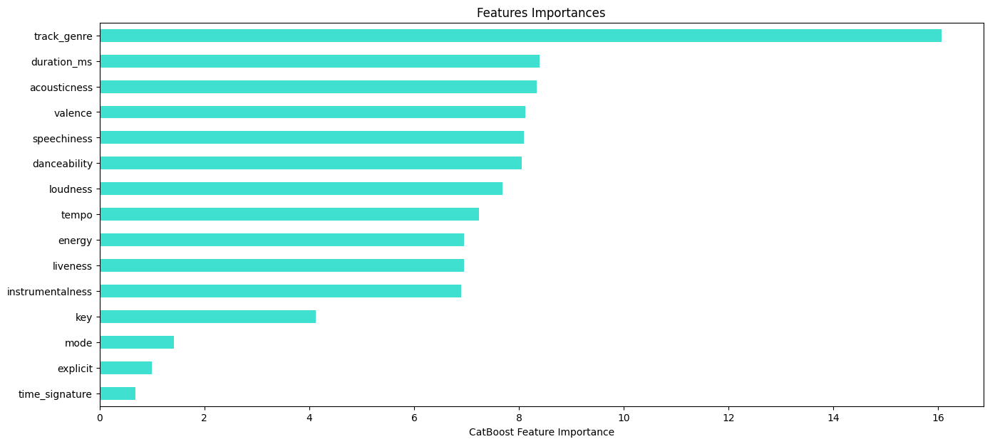
Feature importance plots and loss metrics can be used to determine whether or not a feature is necessary. Removing unecessary features makes the model more interpertable and reduces overfitting.
Feature importance.
importances = pd.Series(data=model.feature_importances_,
                        index= X_train.columns)
importances_sorted = importances.sort_values()
importances_sorted.plot(kind='barh', color='turquoise')
plt.xlabel("CatBoost Feature Importance")
plt.title('Features Importances')
plt.show()
Loss plot.
model.get_all_params()

summary = model.select_features(
    train_dataset,
    eval_set=test_dataset,
    features_for_select='0-14',
    num_features_to_select=10,
    steps=3,
    train_final_model=False,
    logging_level='Silent',
    plot=True
)

summary
Final Model
Create final model with relevant features and optimized parameters.
dataframe = music_data[['popularity_code', 'duration_ms', 'danceability', 'energy', 'key', 'loudness', 'speechiness', 'acousticness', 'instrumentalness','liveness', 'valence', 'tempo', 'track_genre']]


X = dataframe.loc[:, dataframe.columns != 'popularity_code']
y = dataframe.loc[:, dataframe.columns == 'popularity_code']


X_train, X_test, y_train, y_test = train_test_split(X, y, test_size=0.3, random_state=13)

categorical_features = ['track_genre']

train_dataset = Pool(X_train, y_train, categorical_features)
test_dataset = Pool(X_test, y_test, categorical_features)


model = cb.CatBoostClassifier()

grid = {'iterations': [800],
        'learning_rate': [0.1],
        'depth': [8],
        'l2_leaf_reg': [4]}

model.grid_search(grid, train_dataset)
Final accuracy numbers.
y_pred = model.predict(X_test)

# Generate the confusion matrix and classification report
print(confusion_matrix(y_test, y_pred))
print(classification_report(y_test, y_pred))

# Display the confusion matrix using ConfusionMatrixDisplay
disp = ConfusionMatrixDisplay(confusion_matrix=confusion_matrix(y_test, y_pred), display_labels=["unpopular", "popular"])
disp.plot(cmap="Blues", values_format="d")
plt.show()
Accuracy metrics:
| precision | recall | f1-score | support | |
|---|---|---|---|---|
| unpopular | 0.82 | 0.81 | 0.82 | 17182 |
| popular | 0.81 | 0.82 | 0.82 | 17018 |
| accuracy | 0.82 | 34200 | ||
| macro avg | 0.82 | 0.82 | 0.82 | 34200 |
| weighted avg | 0.82 | 0.82 | 0.82 | 34200 |
Interpreting Model
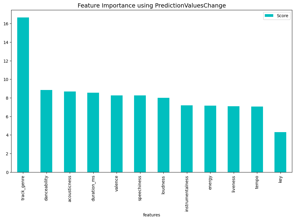
Examine features using feature importances, prediction values change, loss values change and interaction effects.
categorical_features_indices = [11]

def permutation_importances(model, X, y, metric):
    baseline = metric(model, X, y)
    imp = []
    for col in X.columns:
        save = X[col].copy()
        X[col] = np.random.permutation(X[col])
        m = metric(model, X, y)
        X[col] = save
        imp.append(m-baseline)
    return np.array(imp)

def get_feature_imp_plot(method):

    if method == "ShapeValues":
        shap_values = model.get_feature_importance(Pool(X_test, label=y_test,cat_features=categorical_features_indices),
                                                                     type="ShapValues")
        shap_values = shap_values[:,:-1]
        shap.summary_plot(shap_values, X_test)

    else:
        fi = model.get_feature_importance(Pool(X_test, label=y_test,cat_features=categorical_features_indices),
                                                                     type=method)

    if method != "ShapeValues":
        feature_score = pd.DataFrame(list(zip(X_test.dtypes.index, fi )),
                                        columns=['Feature','Score'])

        feature_score = feature_score.sort_values(by='Score', ascending=False, inplace=False, kind='quicksort', na_position='last')

        plt.rcParams["figure.figsize"] = (12,7)
        ax = feature_score.plot('Feature', 'Score', kind='bar', color='c')
        ax.set_title("Feature Importance using {}".format(method), fontsize = 14)
        ax.set_xlabel("features")
        plt.show()
Show plots.
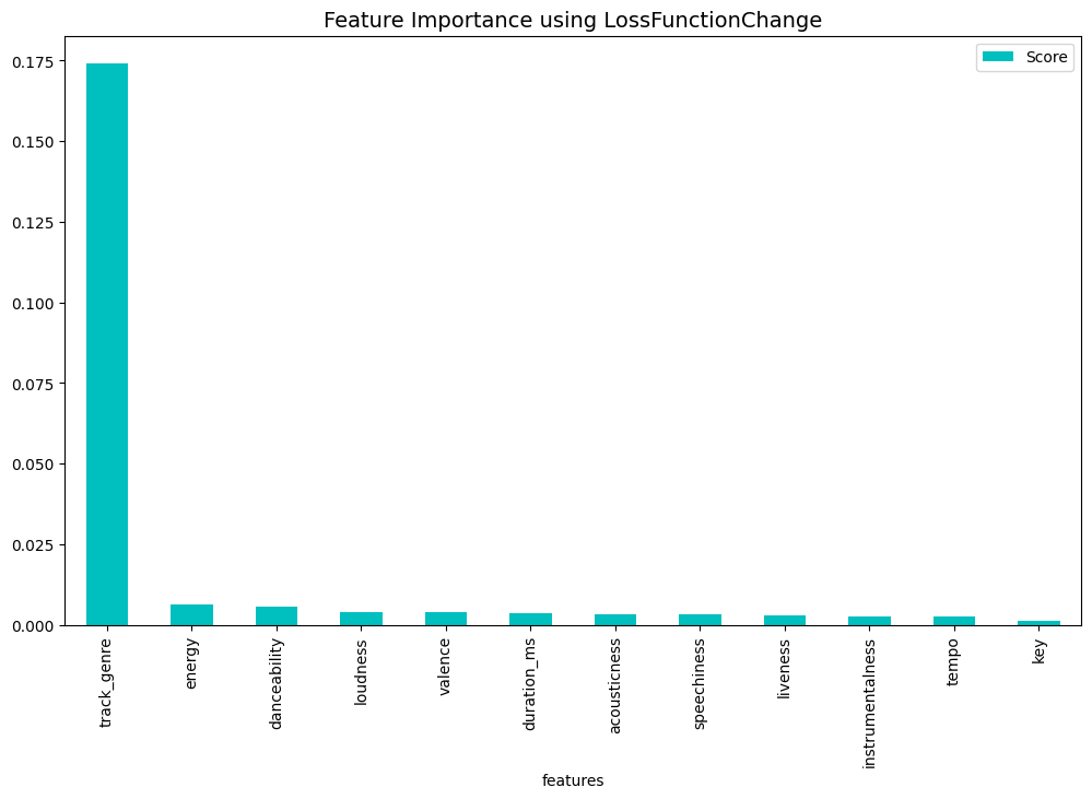
print(get_feature_imp_plot(method="PredictionValuesChange"))
print(get_feature_imp_plot(method="LossFunctionChange"))
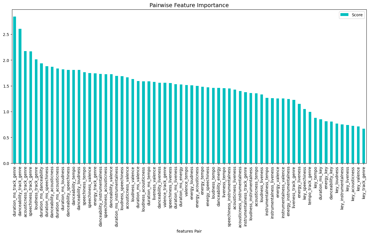
fi = model.get_feature_importance(Pool(X_test, label=y_test,cat_features=categorical_features_indices),
type="Interaction")
fi_new = []
for k,item in enumerate(fi):
first = X_test.dtypes.index[fi[k][0]]
second = X_test.dtypes.index[fi[k][1]]
if first != second:
fi_new.append([first + "_" + second, fi[k][2]])
feature_score = pd.DataFrame(fi_new,columns=['Feature-Pair','Score'])
feature_score = feature_score.sort_values(by='Score', ascending=False, inplace=False, kind='quicksort', na_position='last')
plt.rcParams["figure.figsize"] = (16,7)
ax = feature_score.plot('Feature-Pair', 'Score', kind='bar', color='c')
ax.set_title("Pairwise Feature Importance", fontsize = 14)
ax.set_xlabel("features Pair")
plt.show()
Examine interaction plot.
Cross Validation
Perform k-fold cross validation to ensure consistent accuracy and loss values.
params = {"iterations": 800,
          "depth": 8,
          "loss_function": "Logloss",
          "verbose": False}

scores = cv(test_dataset,
            params,
            fold_count=5,
            plot="True")
Output:
Training on fold [0/5]

bestTest = 0.4475915
bestIteration = 799

Training on fold [1/5]

bestTest = 0.4531492558
bestIteration = 799

Training on fold [2/5]

bestTest = 0.4530666369
bestIteration = 799

Training on fold [3/5]

bestTest = 0.4409488215
bestIteration = 799

Training on fold [4/5]

bestTest = 0.4597720575
bestIteration = 799
Save Model
Save model to use for making predictions on new data.
model.save_model('spotify_random_forest/music_model',
           format="cbm",
           export_parameters=None,
           pool=train_dataset)
Conclusion
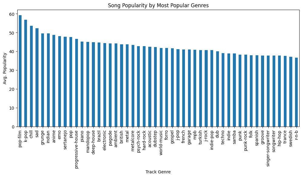
In conclusion, the CatBoost classification model was able to predict whether or not a song was popular or not with 82% accuracy. Track genre appeared to be the strongest predictor of song popularity with the top three most popular genres being “film-pop”, “k-pop” and “chill”.
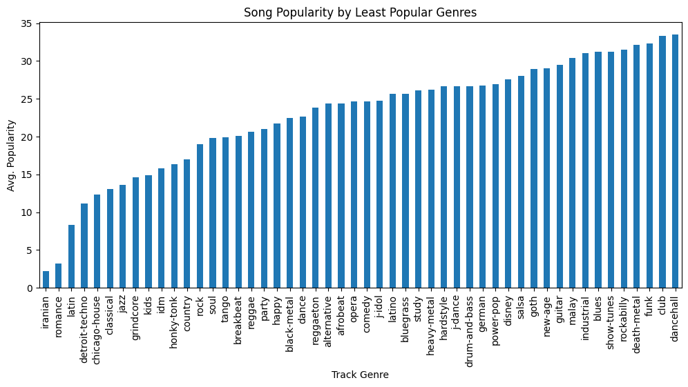
The three least popular genres are “Iranian”, “romance” and “Latin”.
The interaction between track genre and length of song (duration), in addition to the interaction between track genre and dancability, were also important features.
