
Image Classifier Crash Course Using Fastai and Pytorch
Image Classification: Background
Image classification is a widely used type of machine learning with numerous practical applications ranging from face recognition (security) to medical image analysis (diagnostic) to wildlife monitoring (conservation). Convolutional neural networks (CNNs) are frequently used for image classification, in part because of the easy-to-use and well-supported TensorFlow and PyTorch python packages. Additionally CNNs require very little data pre-processing (feature extraction is automated), making them an ideal choice for image classification problems.
- Image Classification: Background
- Neural Network Overview
- Convolutional Neural Network: An Example Using Fastai (Pytorch)
- A Note About Tensors
- Final Thoughts: Deploy as a Web Application
Neural Network Overview
As the name suggests, neural network computational models are inspired by the way biological neural networks function in the human brain, specifically the connectivity patterns of neurons in the visual cortex. A neural network learns to map input data to output predictions by adjusting the weights and biases through a training process, specifically feeding data forward through the network, evaluating the prediction’s error, and iteratively refining the network’s parameters to improve performance.
Key Concepts
There a several key concepts that give a neural network its ability to learn and predict. First, weights (also called parameters) are assigned and automatically tested against a true value (actuals or labels). The error (loss) between the weight performance (predictions) and the actual values (labels) is calculated to iteratively test the weights/parameters, allowing for the selection of weights that yield the highest accuracy.
The architecture of the CNN model consists of an input layer, one or more hidden layers, and an output layer; the input layer receives the initial data (independent variable), the hidden layers process information, and the output layer produces the final result (predictions). Model performance is evaluated based on loss, or how well the model output (predictions) match up with the correct labels (also called target or dependent variable).
Terms and Definitions
- Neuron (or Node):
- The fundamental unit in a neural network is a neuron. Each neuron takes multiple input signals, processes them, and produces an output.
- Layers: Input, Hidden, and Output Layers:
- Neural networks are organized into layers: an input layer, one or more hidden layers, and an output layer. The input layer receives the initial data, the hidden layers perform mathematical computations, and the output layer produces the resulting prediction.
- Connections: Weights and Biases:
- Each connection between neurons has a weight, which determines the strength of the connection and a bias, which allows for fine-tuning the activation of the neuron. These weights and biases are adjusted during the training process to optimize the network’s performance.
- Activation Function:
- Each neuron typically applies an activation function to the weighted sum of its inputs and bias. Common activation functions include the sigmoid, hyperbolic tangent (tanh), and rectified linear unit (ReLU). Activation functions introduce non-linearity, allowing the network to learn complex patterns.
- Feedforward Process:
- During the feedforward process, data is input into the neural network and it propagates through the layers. Neurons in each layer process the input and pass the result to the next layer until the output layer produces the final prediction or classification.
- Loss Function:
- The output of the neural network is compared to the true or expected output using a loss function. The loss function quantifies the difference between the predicted and actual values.
- Backpropagation:
- Backpropagation is the training process where the network learns from its mistakes. The gradient of the loss with respect to the network’s weights and biases is computed, and the weights and biases are continuously adjusted to minimize the loss. This process is typically performed using optimization algorithms like gradient descent.
- Training and Iteration:
- The neural network iteratively goes through the feedforward and backpropagation processes on the training data until it converges to a state where the loss is minimized. This process allows the network to learn the underlying patterns and relationships in the data.
- Testing and Inference:
- Once trained, the neural network can make predictions or classifications on new, unseen data (test data). During this inference phase, the network utilizes the learned weights and biases to process input and produce output.
Convolutional Neural Network: An Example Using Fastai (Pytorch)
The following example is from the fastbook online course which uses fastai and pytorch. The entire course can be found here https://github.com/fastai/fastbook.
Import packages and set Bing API key.
!pip install -Uqq fastbook
import fastbook
fastbook.setup_book()
from fastbook import *
from fastai.vision.widgets import *

APIKEY='xxx'
key = os.environ.get('AZURE_SEARCH_KEY', APIKEY)
Data Preparation
Get training data from a Bing image search, save images in folder named for label.
wonder_types = 'Christ the Redeemer','Machu Picchu','Taj Mahal', 'Petra', 'Chichen Itza', 'Great Wall of China', 'Roman Colosseum'
path = Path('wonders')

if not path.exists():
    path.mkdir()
    for o in wonder_types:
        dest = (path/o)
        dest.mkdir(exist_ok=True)
        results = search_images_bing(key, f'{o}')
        download_images(dest, urls=results.attrgot('contentUrl'))
Print image paths.
fns = get_image_files(path)
fns
Detect corrupt images.
failed = verify_images(fns)
failed
Remove corrupt images.
failed.map(Path.unlink);
(#9) [Path(‘wonders/Chichen Itza/00000054.jpg’),Path(‘wonders/Chichen Itza/00000004.jpg’),Path(‘wonders/Taj Mahal/00000059.jpg’),Path(‘wonders/Taj Mahal/00000055.jpg’),Path(‘wonders/Taj Mahal/00000133.jpg’),Path(‘wonders/Roman Colosseum/00000082.jpg’),Path(‘wonders/Petra/00000017.jpg’),Path(‘wonders/Machu Picchu/00000110.jpg’),Path(‘wonders/Machu Picchu/00000137.jpg’)]
Create fastai datablock object.
### fastai datablock object
wonders = DataBlock(
    ### what is the IV and DV (lables and inputs)
    blocks=(ImageBlock, CategoryBlock),
    ## function to get list of all filenames
    get_items=get_image_files,
    ### how to split data into validation set and training set
    splitter=RandomSplitter(valid_pct=0.2, seed=42),
    ## how to label the data (uses a predefined function - usually file is in folder according to label)
    get_y=parent_label,
    ## functions that get applied to every image, for example resizing each image
    item_tfms=Resize(128))


dls = wonders.dataloaders(path)
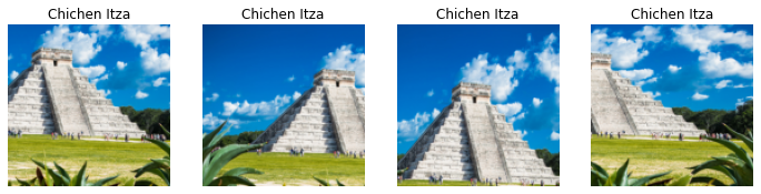
View training data.
### show training data
dls.valid.show_batch(max_n=4, nrows=1)

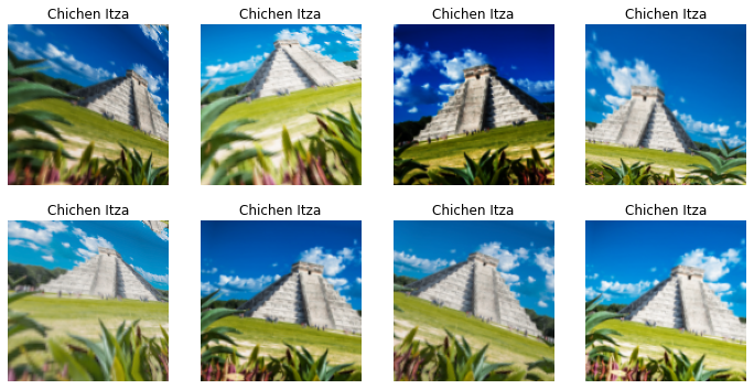
View training data with image cleaning techniques (random resize crop and image augmentation).
### view random resize crop images
wonders = wonders.new(item_tfms=RandomResizedCrop(128, min_scale=0.3))
dls = wonders.dataloaders(path)
dls.train.show_batch(max_n=4, nrows=1, unique=True)
### view data augmentation
wonders = wonders.new(item_tfms=Resize(128), batch_tfms=aug_transforms(mult=2))
dls = wonders.dataloaders(path)
dls.train.show_batch(max_n=8, nrows=2, unique=True)
Apply random resize crop and data augmentation to image data.
### apply random resize crop and data augmentation to your images
wonders = wonders.new(
    item_tfms=RandomResizedCrop(224, min_scale=0.5),
    batch_tfms=aug_transforms())
dls = wonders.dataloaders(path)
Convolutional Neural Network
Create model to recognize images of the 7 wonders of the modern world.
learn = cnn_learner(dls, resnet18, metrics=error_rate)
learn.fine_tune(4)
| epoch | train_loss | valid_loss | error_rate | time |
|---|---|---|---|---|
| 0 | 1.689869 | 0.641205 | 0.177665 | 00:37 |
| epoch | train_loss | valid_loss | error_rate | time |
|---|---|---|---|---|
| 0 | 0.361748 | 0.385056 | 0.106599 | 00:38 |
| 1 | 0.268191 | 0.349137 | 0.096447 | 00:38 |
| 2 | 0.186059 | 0.313965 | 0.086294 | 00:38 |
| 3 | 0.141402 | 0.303486 | 0.081218 | 00:38 |
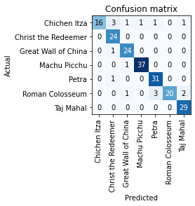
Model Evaluation
Examine accuracy of model using classification matrix.
interp = ClassificationInterpretation.from_learner(learn)
interp.plot_confusion_matrix()
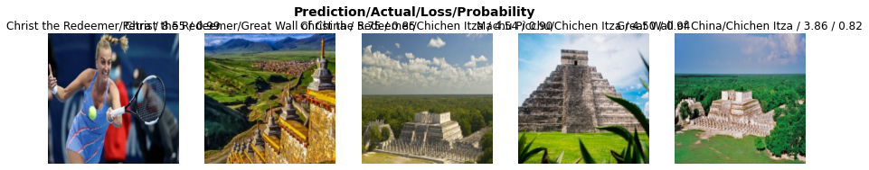
View misclassifications/errors
interp.plot_top_losses(5, nrows=1)
Test Model on New Data
Export your neural network to upload later for image clasification tasks in a production environment using python pickle.
learn.export()
path = Path()
path.ls(file_exts='.pkl')
learn_inf = load_learner(path/'export.pkl')
Try out several test images to see how the model works.
# ims = ['https://en.wikipedia.org/wiki/Machu_Picchu#/media/File:Machu_Picchu,_Peru.jpg']
# dest = '/content/machupicchu.jpg'
# download_url(ims[0], dest)
im = Image.open('colosseum.jpg')
im.to_thumb(128,128)

learn_inf.predict('colosseum.jpg')
(‘Roman Colosseum’, tensor(5), tensor([2.6308e-03, 2.9934e-05, 8.6608e-04, 1.3300e-04, 5.8481e-02, 9.3752e-01, 3.3600e-04]))
Use .vocab to examine labels of tensors from the prediction output (printed above).
learn_inf.dls.vocab
[‘Chichen Itza’, ‘Christ the Redeemer’, ‘Great Wall of China’, ‘Machu Picchu’, ‘Petra’, ‘Roman Colosseum’, ‘Taj Mahal’]
A Note About Tensors
A tensor is a type of multimathematical representation of an object that obeys certain rules during transformation that make them useful for storing and predicting multilinear relationships.
Tensor dimensionality can be described using rank. A tensor of rank 0 is simply a number, a rank 2 tensor is a vector, a rank 3 tensor is a 2 dimensional matrix and a rank 4 tensor is now a 3 dimensional object; tensors can be different multidimensional geometric shapes and this allows them to store information about complex multilinear relationships.
A tensor is the data structure used for convolutional neural networks (the input of a CNN is an image represented as a tensor, as is the output). Tensors in a CNN flow through the network, transforming from input tensors representing raw data to output tensors providing predictions. The input tensor is transformed through convolutional layers with the application of filters and feature extraction (called feature or activation maps), and activation layers (e.g., ReLU), such that the spatial and feature information of the input is retained.
The tensor then undergoes a dimensionalty reduction process (pooling), is flattened into 1D array that passes through one or more fully connected layers where features are extracted to the desired output classes. The final tensor represents the network’s prediction scores (and probability) for each class. As seen in the example above, the predicted class is the one with the highest probability.
Final Thoughts: Deploy as a Web Application
In summary, augmented/resized training data obtained from Bing search engine can be used with the fastai python package to create a simple and effective convolution neural network for image classification.
While code for the neural network is sufficient for accessing and validating the model, it may be helpful to demonstrate the efficacy of the model in a simple user interface - this will allow others to easily test the model and potentially assist with prototyping. Python’s flask package is a fast and simple way to create a web application where others will be able to use your image classification model, and can be deployed for free using fly.io.
Visit this link to test out the convolutional neural network created using the above code from this article (please allow about 30 seconds for the model to load). See the full code for the Flask application in this github repo.
The citation for the above example provided here:
Deep Learning for Coders with Fastai and Pytorch: AI Applications Without a PhD, by Howard, J. and Gugger, S., isbn: 9781492045526, url: https://books.google.no/books?id=xd6LxgEACAAJ, year: 2020, publisher: O’Reilly Media, Incorporated
