
Comparing Classification Techniques using Human Movement Data
Introduction
Classification - teaching a model to recognize patterns and assign labels to new examples - is a fundamental machine learning problem. Decision trees and neural networks are two well-established techniques for tackling classification tasks. Now with the rise in popularity of large language models (LLMs) there is another new, popular approach. Each method brings its own strengths, limitations, and assumptions about the data.
In brief, decision trees provide an interpretable, rule-based way of splitting and classifying the data. Neural networks also excel at capturing complex nonlinear patterns in high-dimensional input for classification tasks. Large language models, though designed for text generation, can be theoretically adapted as powerful general-purpose classifiers. I’ll implement each of these methods, measure how well they predict movement type, and compare their accuracy side by side to see which technique best fits this problem.
Data Preparation
The data to compare three different classification approaches (decision trees, neural networks, and LLMs) were sourced from the WISDM Smartphone and Smartwatch Activity and Biometrics dataset collected by researchers at Fordham University’s Wireless Sensor Data Mining (WISDM) Lab in New York. ARFF files containing sensor readings from both phones and watches across accelerometer and gyroscope sensors are available on Kaggle.
The data was collected to represent a large-scale, realistic dataset of human motion that could be used to advance research in activity recognition (e.g., detecting whether someone is walking, jogging, climbing stairs, etc.) and biometric identification (using patterns of movement to recognize individuals). It contains motion sensor data collected from 51 subjects using both a smartphone (in the pocket) and a smartwatch (on the dominant wrist) and contains data from 18 different activities, including walking, jogging, climbing stairs, eating, brushing teeth, and playing catch, with each activity lasting three minutes. The dataset includes raw accelerometer and gyroscope readings from both devices, sampled at 20Hz, totaling over 15 million measurements. The researchers transformed this raw data into labeled examples using a sliding window approach, creating high-level features suitable for machine learning models.
For each subject, the code loads the corresponding four ARFF files, converts them to pandas DataFrames, standardizes column names, and prefixes feature columns by device and sensor type to avoid naming collisions.
BASE_PATH = "~/code/human_movement/data/wisdm-dataset/wisdm-dataset/arff_files"

DEVICES = ["phone", "watch"]
SENSORS = ["accel", "gyro"]

def load_subject_data(subject_id):
    dfs = []
    for device in DEVICES:
        for sensor in SENSORS:
            sensor_dir = os.path.join(BASE_PATH, device, sensor)
            filename = f"data_{subject_id}_{sensor}_{device}.arff"
            filepath = os.path.join(sensor_dir, filename)

            if os.path.exists(filepath):
                df = load_arff_to_df(filepath)
                df.columns = [col.strip('"') for col in df.columns]
                df = prefix_columns(df, f"{device}_{sensor}")
                dfs.append(df)
            else:
                return None  # skip subject if missing

    df_merged = pd.concat([
        dfs[0],
        dfs[1].drop(columns=["ACTIVITY", "class"]),
        dfs[2].drop(columns=["ACTIVITY", "class"]),
        dfs[3].drop(columns=["ACTIVITY", "class"]),
    ], axis=1)

    return df_merged
The sensor DataFrames are then horizontally concatenated under the assumption that rows are time-aligned, preserving a single set of activity labels. Data from all valid subjects are vertically combined into one dataset, dropping any subjects with missing values. The final cleaned dataset is exported as a single CSV file.
Decision Trees
A Random Forest (or any tree-based ensemble model) is usually an excellent starting point for most classifications problems with tabular data; trees are very forgiving when it comes to assumptions about your data so they typically require little preprocessing before getting baseline accuracy statistics (read more about supervised learning and tree-based models here: https://cfrench575.github.io/posts/spotify-boosted-decision-trees/#tree-based-models) The scikit-learn python package can be leveraged to quickly train and evaluate a Random Forest.
# Encode predicted/target variable
le = LabelEncoder()
df["ACTIVITY_LABEL"] = le.fit_transform(df["ACTIVITY"])

# Split features and target
X = df.drop(columns=["ACTIVITY", "class", "ACTIVITY_LABEL"])
y = df["ACTIVITY_LABEL"]

# Split into train/test sets
X_train, X_test, y_train, y_test = train_test_split(
    X, y, stratify=y, test_size=0.2, random_state=42
)

# Create pipeline (scaling + classifier)
pipeline = Pipeline([
    ("scaler", StandardScaler()),  # scales numeric features
    ("clf", RandomForestClassifier(n_estimators=100, random_state=42))
])

# Train model
pipeline.fit(X_train, y_train)
model = pipeline.named_steps['clf']

# Predict test
y_pred = pipeline.predict(X_test)
Random Forest Results: Confusion Matrix
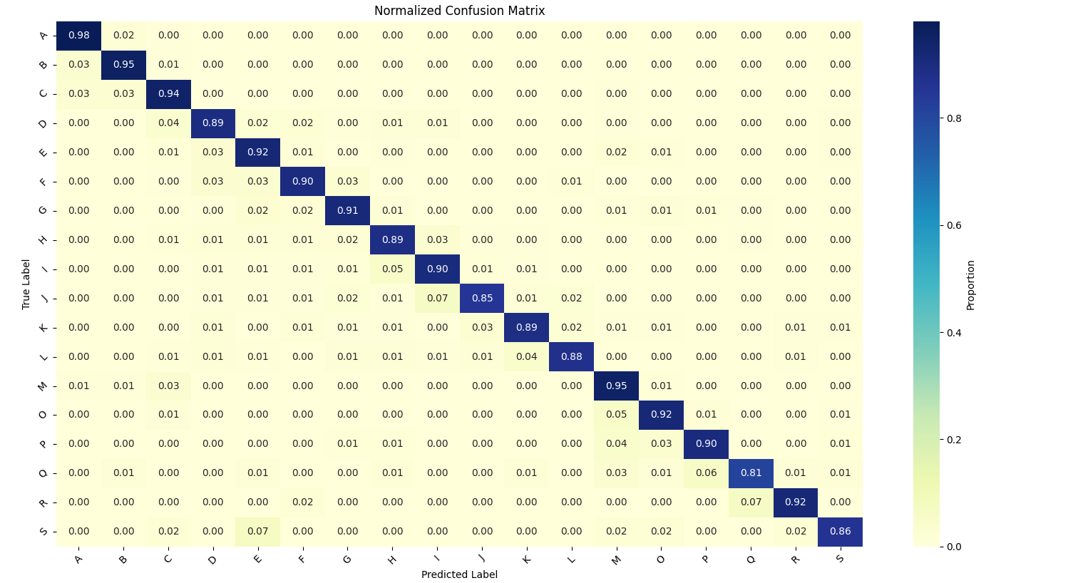
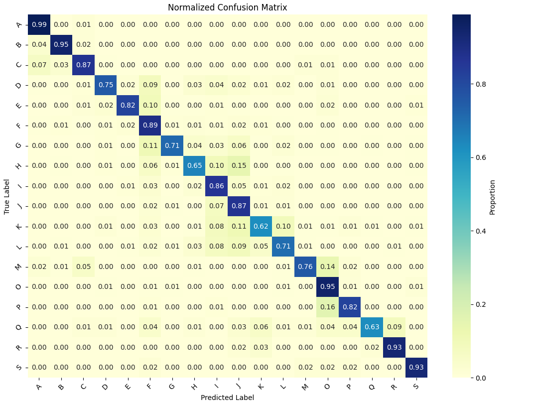
After your model has been trained and predicitons for the test set have been created, a color-coded confusion matrix can be used to quickly visualize how well the random forest model was able to predict human movement type based on the smartphone and smartwatch data.
In this case since there are 18 movements to classify (a high number of groups) with class imbalances (ranging from 57 to 263 participants), I’ve plotted normalized proportions of cases instead of the raw values. Right out the gate the random forest is able to effectively classify movements based on the smartphone and smartwatch gyroscopic data, with an overall accuracy of 91%.
Random Forest Results: Feature Importances
A random forest is also comparatively more interpertable than LLMs and neural network. Scikit-learn models have a feature importances attribute model.feature_importances_ that can be easliy accessed, sorted and ploted in a bar chart. For this random forest model, the most important feature for predicting movement type is
phone_accel_YABSOLDEV and phone_accel_YSTANDDEV, two measures of variation in vertical movement.
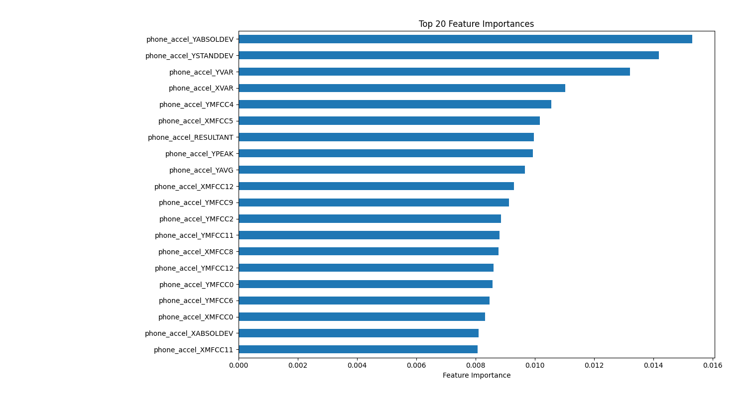
An additional measure of feature influence available in scikit-learn is permutation importance result = permutation_importance(model, X_test, y_test, n_repeats=10, random_state=13) Permutation feature importances are calculated by randomly shuffling/randomizing each single feature’s values and capturing the corresponding change in overall accuracy of the model. phone_accel_YABSOLDEV (variation in vertical movement) and phone_accel_XVAR (variance in side-to-side motion) are the most influential measures based on permutation importance.

Random Forest Results: SHap Values
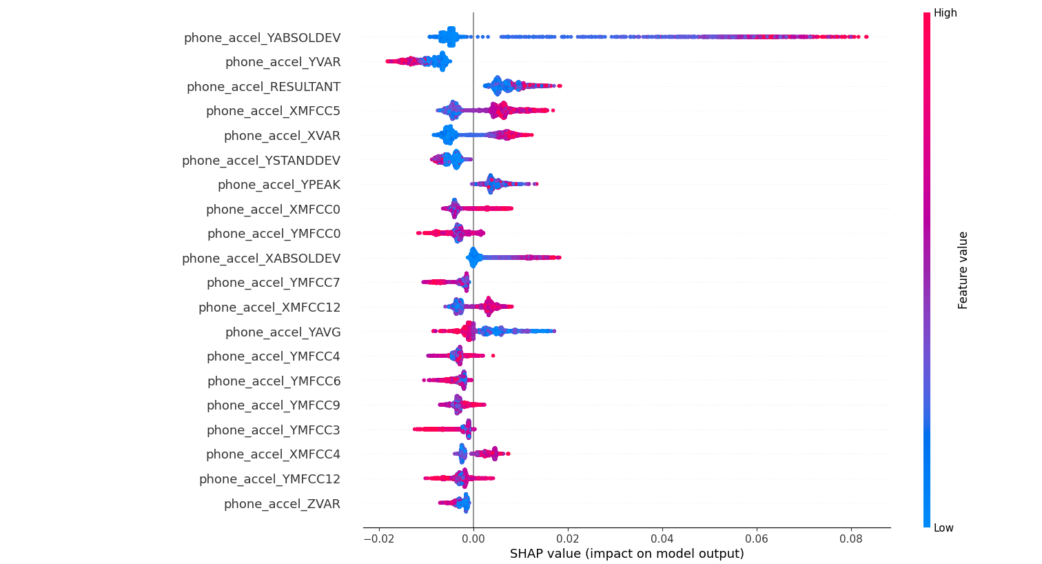
For a detailed, highly interpertable examination of feature importance, calculating and plotting feature shap (SHapley Additive exPlanations) values can provide insight into both global (across all predictions) and local (for a single prediction) feature importances. Derrived from game theory, each feature’s SHAP value is like its “fair share” of responsibility for moving the prediction away from the baseline (average) prediction. Positive SHAP values push the prediction higher, while negative ones push it lower. The visualization of shap values clearly shows that the feature phone_accel_YABSOLDEV has a strong infulence on model predictions, particularly at higher values.
Random Forest Results: LIME Explainer
Lastly, for comprehensive explainability for a single prediction, the LIME (Local Interpretable Model-agnostic Explanations) python package can be applied to any machine learning model. To generate an explanation for a specific prediction LIME trains a simple, interpretable model like linear regression on perturbed samples by modifying features and measuring resulting prediction changes with only a few lines of code:
from lime.lime_tabular import LimeTabularExplainer
explainer = LimeTabularExplainer(training_data=X_train.values, feature_names=X_train.columns, class_names=model.classes_, mode="classification")

# explanation for a single prediction at index
exp = explainer.explain_instance(X_test.iloc[0].values, model.predict_proba)
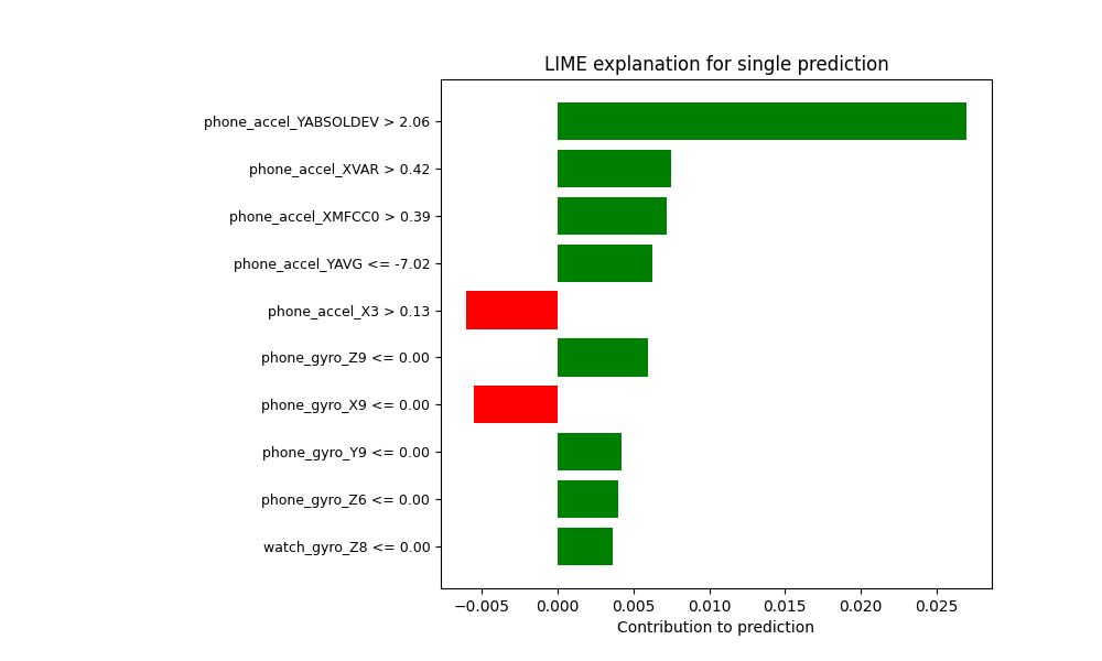
In a LIME explanation, the weights can be positive or negative, and they tell you whether a feature is pushing the prediction toward the predicted class or away from it. Positive weights indicate the feature value contributes in favor of the selected class, whereas negative weights indicate the feature contributes against the model predicting that class. Plotting these values we can see a visual representation of the weights for this particular prediciton, and conclude that having phone_accel_X3 > 0.13 slightly decreases the likelihood of the predicted activity class.
Random Forest Results: Conclusions
In summary, using scikit-learn’s random forest classifier trained on cleaned smartwatch and smartphone tabular movement data can classify 18 movement types with 91% accuracy, without extensive feature scaling or parameter tuning. Additionally, there are several simple functions available to quickly perform complex calculations to assess feature importance and feature impact on the model across all predicitons, or for a single individual prediction. This is the typical and recommended strategy for classification tasks, and in this case yields both high accuracy and high interpertability.
Neural Networks
Less interpertable than tree models but able to fit to more complex patterns, a neural network is another candidate for creating a classifier. Below is a basic example for initial testing of the classification ability of a neural network using python’s tensorflow. With two hidden layers (128 and 64 nodes), the network hopefully has enough representational power to capture complex patterns in the data without being so large that it immediately risks overfitting. The output layer has 18 nodes/neurons to represent the 18 activity classes being predicted. The adam optimizer is fast to converge, stable, and therefore a good starting place, and the loss function sparse categorical crossentropy is the appropriate choice for predicting categorical features represented as integers in the data.
from tensorflow.keras.models import Sequential
from tensorflow.keras.layers import Dense


X_train, X_test, y_train, y_test = train_test_split(
    X, y, stratify=y, test_size=0.2, random_state=42
)

model = Sequential([
    Dense(128, activation='relu', input_shape=(364,)),
    Dense(64, activation='relu'),
    Dense(18, activation='softmax')
])

model.compile(optimizer='adam', loss='sparse_categorical_crossentropy', metrics=['accuracy'])

model.fit(X_train, y_train, epochs=10, batch_size=32)

y_pred_probs = model.predict(X_test)
y_pred = np.argmax(y_pred_probs, axis=1)
This neural network was able to classify action type from recorded movements with 82% accuracy
Neural Network Results: Confusion Matrix
Neural Network Results: Conclusions
Neural networks are generally considered less interpertable than tree models, and there are no built in functions to calculate feature importances or summary shap values for a multiclass (18 classes) classification model like this one. Using the neural network not only resulted in a less accurate model 91% versis 82% accuracy, but also limited the number of data explainability tools that can be used to interpert the model. At this point if I really preferred to use a neural network over a random forest, I would wrap the model in a Python class that inherits from sklearn.base.BaseEstimator so that it could function as a scikit-learn estimator.
Large Language Models
How does a large language model compare to more traditional machine learning methods for a classification task? The first limitation that becomes evident is the small token count for free models available at https://openrouter.ai. To apply an LLM to this classificaiton task, I first round the decimal values which puts me at about 2000 tokens per row. I subset only 400 out of the over 16000 rows in the human movement dataset (300 rows for training, 100 rows for testing) which eats up the entire 1 million token context window and creates a significant data quality concern. After formatting the training and test data as strings, the code used to retrieve LLM predicitons for the test set is below:
prompt = f"""
You are a classifier based on Training examples: {train_examples}

predict 'ACTIVITY' for each of the 90 test cases: {test_cases}

output is a list of ACTIVITY predictions there should be one for each of the 90 test cases. The order of the list should match the order of the test cases. The list should have exactly 90 predictions.
"""

# prompt = test_cases
encoding = tiktoken.get_encoding("cl100k_base")
token_count = len(encoding.encode(prompt))

OPENROUTER_API_KEY = "my-free-key-here"
# https://openrouter.ai/google/gemini-2.0-flash-exp:free/api -- 1M context window


client = OpenAI(
  base_url="https://openrouter.ai/api/v1",
  api_key=OPENROUTER_API_KEY,
)

completion = client.chat.completions.create(
  extra_body={},
  model="google/gemini-2.0-flash-exp:free",
  messages=[
    {
      "role": "user",
      "content": prompt
    }
  ]
)
print(completion.choices[0].message.content)

## extract list
match = re.search(r"\[.*\]", completion.choices[0].message.content, re.S)
if match:
    predictions = ast.literal_eval(match.group(0))


sampled_test['llm_classifications'] = predictions
sampled_test.to_csv('llm_test_predictions.csv')
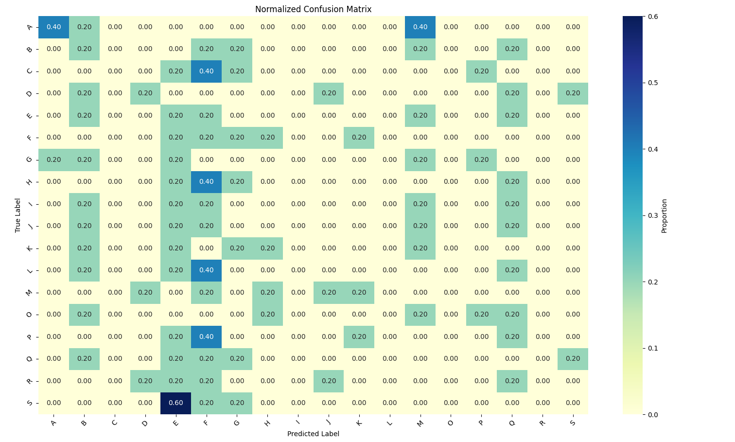
Large Language Model Results: Confusion Matrix
Plotting a normalized confusion matrix of the test predictions, it’s immediately evident that the LLM could not predict movement type with any sort of accuracy. Additionally, this is the least transparent classification method demonstrated so there is no process for getting insight into how the LLM used the training data and therefore diagnose where it might have gone wrong.
Large Language Model Results: Conclusions
Using an LLM for classification tasks will be needlessly expensive and difficult to interpret. For this problem the LLM could not process all the data due to context limits, and truncating decimals caused information loss. Accuracy was low (next to zero) and reasoning was impossible to evaluate or replicate. I had to specify the number of predictions to return, which ate into my precious context window, because the model’s initial outputs didn’t seem match the test cases. Overall, the number of practical challenges and low accuracy make it an undersirable method for classification problems, especially when a random forest or neural network model appears immediately effective.
Conclusion
Data Science is an exciting and rapidly changing domain; when I started my career data science-specific degrees didn’t even exist yet. In a short amount of time the field has evolved from statistics and business intelligence reporting, to predictive machine learning modeling, to deep learning, to large language models, and now to agentic systems.
With the current ubiquity of LLMs investors and nontechnical leadership can be tempted to throw this black-box technique at all data products; when a large language model is the shiniest hammer in the toolbox, every data problem gets contorted until natural language generation is the solution. But an experianced data scientist understands that a more complicated technique is not a substitute for intelligent, planned, domain-specific training data. Sacrificing interpretability and replicability for expensive state-of-the-art LLMs is unlikely to yeild higher accuracy - it will likely result in higher expenses for processing excessive amounts of tokens and a headache that comes with sending potentially proprietary data to an outside party.
When is it appropriate to use an LLM? The standards for LLM evaluation and performance are still being set, and context engineering is becoming an increasingly important technique to address some of the known LLM limitations. Products are also moving away from a single, general LLM that is expected to perform any task to multiple smaller, specialized LLMs working in tandem to form an agentic system. It’s a powerful tool with a growing number of applications, but out-of-the-box it is likely to underperform on highly specific classification tasks compared to most other ‘simplier’ data modeling techniques that leverage relevant context and high quality training data.
